Target Audience: HES operators, SCADA engineers, energy company managers
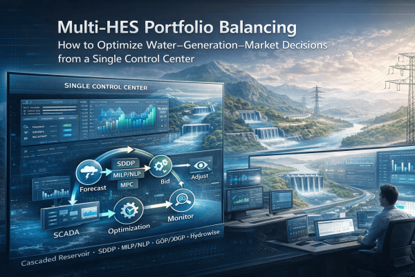
Multi-HES Portfolio Balancing: How to Optimize Water–Generation–Market Decisions from a Single Control Center
Hook + problem definition
Same river basin, same rainfall regime, similar turbine efficiencie yet you can see a striking gap between the monthly revenue lines of two companies running a “multi-HES portfolio.” The reason is simple: in portfolio management, what matters is not only how much you generate, but which plant, in which hours, under which water constraints, and with which market position you operate. Optimizing each HES separately often produces a “local optimum”; in a cascaded (sequential reservoir) structure, that approach can cause a decision made upstream to come back downstream as spill or a missed opportunity [6]. This article lays out an advanced but practical framework for managing a multi-HES portfolio from a single control center covering the portfolio concept, constraints, and objective function. [6]
TL;DR
- Portfolio balancing is not single-plant optimization; it is maximizing total value under a shared water resource + shared constraints + shared risk [1][6].
- In cascaded HES, the core game is aligning water value (water value) and the price profile in one objective function and minimizing spill [1][6].
- The most robust architecture in practice is multi-layer optimization: long-term water policy (SDDP) + short-term unit/production scheduling (MILP/NLP) + near real-time correction (MPC) [1][2][4][8].
- “Market bidding” (GÖP/GİP/DGP) is essentially the output of portfolio optimization: generation plan + adjustment band + flexibility option [7][11].
- A data-driven approach connects forecasting, SCADA data, and optimization into a single decision loop, enabling proactive rather than reactive portfolio management.
What is a portfolio (in the HES context)?
A portfolio is the framework in which multiple generation assets operated by the same company (or the same control center) are managed with a total risk return perspective. In hydro, “portfolio” typically means:
- Managing storage and flow dynamics across multiple dams/reservoirs together,
- In a cascaded structure, upstream discharge becoming the downstream “inflow,”
- The generation function changing nonlinearly with head and efficiency [4][5],
- Market prices being uncertain, and hydro generation behaving like an option due to its ability to shift production in time [7].
In a hydro portfolio, the “inventory” (water) is time-dependent. Generating less and saving water today is effectively an investment decision that grants you the right to generate in tomorrow’s high-price hours. That is why hydro planning is naturally a multi-stage optimization problem [1].
Constraints: what makes it a single “portfolio problem”
Key constraint classes that make multi-HES optimization both challenging and valuable:
- Water balance and reservoir limits: storage min/max; inflow, outflow, spill, and environmental minimum flows [1][6].
- Cascade/hydraulic coupling: upstream releases feed downstream plants; poor timing can increase spill in lower basins [6].
- Head and efficiency sensitivity: generation depends not only on discharge but also on reservoir level–head–turbine curves. Some problems are modeled via piecewise linear MILP, others via direct NLP [4][5].
- Unit constraints and operating security: start/stop, minimum up/down, ramping, maintenance windows; mode switching in pumped storage [4][10].
- Market and operational constraints: a plan in GÖP, corrections in GİP, flexibility in DGP; gate closures and activation risk (operational “commitment risk”) [7][11].
Objective function: more than “profit”
In advanced portfolio balancing, the objective is rarely a single sentence. In most real systems, it is a weighted combination of:
- Maximize expected revenue/profit: price × generation, with bidding strategy aligned to the schedule [7][11].
- Minimize spill and water waste: improves cascade efficiency [6].
- Reduce imbalance/deviation cost: driven by uncertainty and commitment risk [11].
- Add risk measures like variance / CVaR according to risk appetite: price and inflow uncertainty [1][3].
- If multi-purpose water use exists (irrigation/drinking water/flood control): model via penalty terms [12].
In hydro planning literature, SDDP is critical for long-term, uncertainty-aware multi-stage optimization because it scales effectively [1][2]. In the short term, detailed unit constraints and head effects are captured with MILP/NLP [4][5]. In practice, the “best approach” is rarely one algorithm; it is a multi-layer chain.
How does it work?
Let’s modularize the “single control center” approach so it works in the field:
Portfolio → Constraints → Objective function → Outputs (plan/bid/dispatch).
Step 1 Model the portfolio: a shared data dictionary
The first requirement for a control center is that all plants “speak” the same portfolio data model:
- Reservoir levels, inflow forecasts, discharge limits
- Unit states, efficiency curves, maintenance constraints
- SCADA measurements (kW, discharge, gates, condition signals like vibration/temperature)
- Market price forecasts and scenarios
Infographic Content (Figure-1): “Portfolio Decision Loop”
Data (SCADA + hydrology + price) → Forecast → Scenario → Optimization → Plan/Bid → Monitoring → Adjustment
This loop is consistent with the approach of integrating decision-support components into SCADA systems for cascaded HES management [9].
Step 2 Layer constraints: make the problem solvable
A single giant optimization model can be “beautiful in theory” and “hard in practice.” Layering constraints is common:
- Long term (weekly/monthly): storage targets, water value, energy budget (with uncertainty) [1][2].
- Short term (hourly/daily): unit loading, head/efficiency, minimum operation, cascade flow matching [4][5][6].
- Near real time: deviation correction, short-horizon re-optimization (MPC) [8].
In cascaded portfolios, being too aggressive with upstream decisions in the short term can magnify spill risk downstream. Short-term planning should remain consistent with long-term water value/policy [1][6].
Step 3 Build the objective: a one-line “portfolio KPI”
A readable objective for a control center is:
Step 4 Translate outputs into “market + operations” language
Optimization output should not be a single table; it should become three product-ready outputs:
- Core plan for GÖP: next-day hourly generation and bid recommendation [7][11]
- Adjustment band for GİP: when and how much to correct as new information arrives [11]
- Flexibility option for DGP: which units can ramp up/down and how fast; offered band based on activation probability [8][10]
Impact on the HES / power plant side (H2)
How does a “portfolio decision” show up in the plant?
On the ground, portfolio balancing directly affects:
- Reservoir level targets: the operational translation of “hold today, sell tomorrow” [1].
- Unit stress profile: frequent start-stop or aggressive ramping increases failure risk and maintenance load (operational penalty) [4][10].
- Spill and downstream constraints: poor cascade coordination wastes water and can forfeit higher revenue opportunities [6].
- Operations vs trading conflict: trading prioritizes price; operations prioritizes safety. A portfolio KPI unifies both into one objective.
- Plan vs actual alignment: without SCADA feedback the portfolio remains “on paper”; near real-time correction becomes essential [8][9].
Head-aware models can produce better economic results in cascaded systems because the same discharge yields different kWh under different head levels [4][5]. In short: it’s not only “generate at the right hour,” but also “generate under the right head conditions.”
A small forecast error is a “deviation” for one HES. In a 5–10 HES portfolio, the same error multiplies into collateral pressure, operational stress, and imbalance cost. That is why uncertainty management and layered planning become mandatory at portfolio scale [1][3][6].
Example scenario / mini calculation / flow
| Date | Hour | PTF_TL_MWh | HES_A_Plan_MWh | HES_B_Plan_MWh | HES_C_Plan_MWh | Total_Plan_MWh | Not | Source |
|---|---|---|---|---|---|---|---|---|
| 2025-04-29 | 18 | 167.99 | Not in source | Not in source | Not in source | 92.80 | Not in source | 1 |
| 2025-04-29 | 19 | 163.14 | Not in source | Not in source | Not in source | 89.17 | Not in source | 1 |
| 2025-04-29 | 20 | 160.58 | Not in source | Not in source | Not in source | 88.11 | Not in source | 1 |
| 2025-04-29 | 21 | 158.32 | Not in source | Not in source | Not in source | 88.79 | Not in source | 1 |
| 2025-04-29 | 22 | 152.87 | Not in source | Not in source | Not in source | 88.77 | Not in source | 1 |
Table-1
PTF data is taken from EPİAŞ Transparency Platform [13]. Data extraction uses the transparencyEpias package [14].
Scenario: a cascaded portfolio with 3 HES (A upstream, B midstream, C downstream)
Three plants lie on the same river; A’s discharge affects B, and B’s discharge affects C.
Next-day evening prices (18:00–22:00) are expected to be high (price scenarios).
There is inflow uncertainty during the day; additionally, plant B shows a slight upward vibration trend (not a failure, but a risk signal).
Portfolio decision problem: “core + band + option”
Goal: maximize revenue in peak hours while minimizing spill and deviation [6][7].
Core plan for GÖP (next day)
- Shift water from A and B reservoirs gradually into 18:00–22:00 (consider cascade delay).
- If C faces higher downstream spill risk, limit aggressive upstream releases [6].
- For head sensitivity: avoid dropping reservoir levels too much and damaging efficiency (especially in peak hours) [4][5].
A simple revenue model is
Σt Pt · Et
.
But in hydro,
Et
is not constant;
Et=f(Qt,Ht)
and
Ht
depends on reservoir level [4][5].
So “generate when price is high” must be paired with “protect head in that hour.”
Adjustment band for GİP (intraday)
The inflow forecast is updated at noon: 8% lower than expected.
In the GİP band, slightly reduce generation allocated to peak hours; cut even more in low-price hours (save water) [1][6].
If vibration increases in B, reduce B’s loading in some hours and compensate with A or C (operational penalty) [10].
Flexibility option for DGP (near real time)
Treat units that can ramp quickly as an “option.”
With MPC, re-optimize in a short horizon (e.g., 1–2 hours) to generate setpoint suggestions that minimize deviation [8].
If risk signals increase in B, shift flexibility capacity offered to DGP toward A/C (risk-aligned decision).
Infographic:
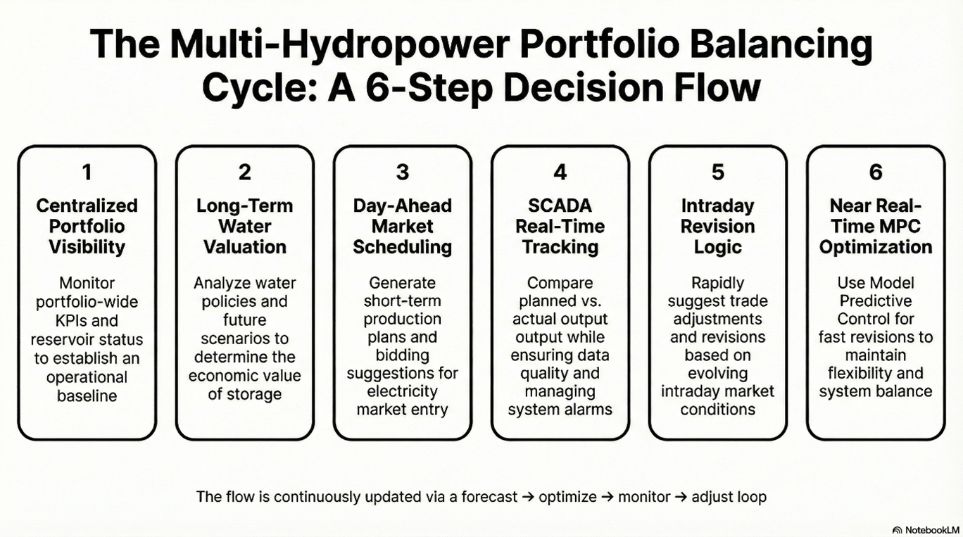
Data-Driven Portfolio Decision Approach
Portfolio balancing is not a one-time plan; it is a continuously evolving decision loop. The objective is to transform fragmented signals into structured decisions: what is changing, what is at risk, and what actions should be taken.
Module 1 Forecast: make price + production uncertainty visible
Price: scenarios (high/medium/low) and uncertainty bands rather than a single point forecast.
Production: an “expected output interval” built from inflow + head/efficiency + maintenance risk.
This supports the co-existence of long-term uncertainty modeling (SDDP) and short-term planning [1][2][3].
Module 2 Portfolio Optimization Engine: a layered solution
Long-term policy: generate water value/policy with SDDP (scalability) [1][2].
Short-term plan: hourly production, unit constraints, head sensitivity via MILP/NLP [4][5].
Near real-time correction: reduce deviation and support economic dispatch via MPC [8].
MILP-based short-term hydro planning often captures head effects via piecewise linear approximations, leveraging solver performance [4]. For head-sensitive cascaded systems, NLP can also be effective [5]. In practice, the product architecture may include both approaches depending on plant type.
Module 3 SCADA/OT integration: close the “plan–actual” loop
In cascaded HES management, integrating decision-support components into SCADA helps combine water management, equipment condition, and operational targets [9]. Product-wise, this becomes:
Measurement → deviation detection → alert/recommendation → approval → setpoint/plan update
Optimization is only as valuable as data quality. Without SCADA tag standardization, time synchronization, and data integrity, the “portfolio model” cannot be trusted. This should be standardized in the product installation checklist.
Module 4 EPİAŞ decision support: plan + band + option screens
To translate portfolio output into “market language,” use a three-screen approach:
- GÖP Bid Recommendation: core plan + water value insight + risk band [7][11]
- GİP Adjustment Recommendation: hourly deviation risk + trade suggestion
- DGP Flexibility Management: activation probability, ramping capability, equipment risk → “offerable flexibility”
Practical MVP: first value in 2–4 weeks
- Week 1: portfolio data dictionary + SCADA core KPIs (kW, discharge, gate, level)
- Week 2: price/production forecast + basic GÖP core plan
- Week 3: GİP adjustment band + alarm thresholds
- Week 4: cascade spill KPI + foundational optimization improvements (MILP vs NLP selection)
FAQs
1) Why isn’t “single plant optimization” enough?
Because in cascades, upstream decisions define downstream inflows; lack of coordination can raise spill and reduce total revenue [6].
2) What is the most critical KPI?
Rather than one KPI, “portfolio value” (revenue – spill – deviation – risk – operational penalty) is more accurate [1][6].
3) Which is better: SDDP or MILP?
It depends on the time horizon. SDDP is strong under uncertainty in the long term [1][2]. MILP/NLP dominates for short-term unit/head details [4][5]. Most systems are hybrid.
4) Is a head-sensitive model mandatory?
It becomes more important as the portfolio grows and reservoir levels vary widely. Including head can improve economics [4][5].
5) How does bidding connect to optimization?
For hydro generators, bidding can be modeled with reservoir status and price dynamics; optimal offering strategies are a classic approach [7]. In Turkey, studies combining wind + pumped storage and optimal offers support portfolio thinking as well [11].
6) What changes with pumped storage (PHES)?
PHES adds time-shifting capability and stronger flexibility; capacity planning and operation must be considered together [10][11].
7) Do metaheuristics (GA, etc.) help in practice?
They can produce fast policies/heuristics for multi-purpose reservoirs under complex constraints [12]. The goal is often “good and feasible,” not guaranteed optimality.
8) Can portfolio balancing work without SCADA integration?
Only in a limited way. Without live feedback, optimization decisions become stale quickly and plan–actual gaps remain open [8][9].
Conclusion + CTA
Multi-HES portfolio balancing is not “watching several plants at once.” It is combining water–generation–market decisions into a single objective function. In cascaded systems, this is one of the most direct ways to reduce spill and increase total revenue [6]. A solid setup ties together long-term water value (SDDP) [1][2], short-term detailed scheduling (MILP/NLP) [4][5], and near real-time correction (MPC) [8], all within a single decision loop supported by Forecast and SCADA integration [9].
If you would like to learn more about portfolio balancing and data-driven decision approaches in hydropower operations, feel free to contact us: