Time-Series Data: How to Store SCADA Data with a Timescale/TSDB Approach (Partitioning, Retention, Query Performance)
As real-time monitoring expands in energy facilities, the question “Are we collecting the data?” quickly turns into “How do we store this data for years and still query it fast?”. On the SCADA side, second-level (or higher-frequency) telemetry continuously streams across hundreds to thousands of tags—kW, flow, gate position, vibration, temperature, and more. Within a few months, row counts can approach the billion scale. At that point, continuing with a classic relational single-table design typically leads to index bloat, query latency, rising costs, and operational maintenance burden.
In this post, we describe the TSDB approach for time-series data and, within the PostgreSQL ecosystem, the Timescale-like “hypertable + chunk” model in the SCADA context. The goal is to keep real-time dashboards fast at millisecond–second scale while storing multi-year archives at a manageable cost. To do that, we cover partition/chunk strategy, retention policies, downsampling (summary data), common query patterns, and performance/operations practices as one coherent system.
1) TL;DR (5 points)
- SCADA data is a “high write volume + time-range queries” problem; time-based partitioning (partition/chunk) is essential [1][2].
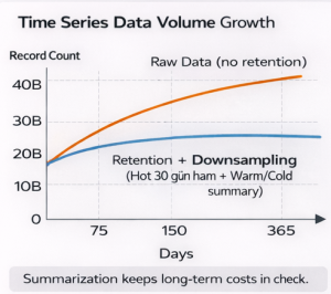
- Keeping everything as raw data forever is not sustainable; you should build the “raw short, summaries long” pyramid with retention + downsampling [3][4].
- The right indexes and the right chunk/partition size determine both ingestion speed and query latency. PostgreSQL declarative partitioning provides the core mechanism [2].
- Most queries collapse into a few patterns: last X minutes trend, time-range aggregation, post-alarm investigation, dashboard KPIs. TSDB design should follow these patterns.
- In Hydrowise, the goal is to store SCADA time series in hot–warm–cold layers, continuously compute KPIs, and keep alarm/analytics screens fast.
2) Concepts and theoretical background
2.1 What is time-series data?
Time-series data is data where each record carries a timestamp and is commonly produced as a stream of sensor/measurement samples. In SCADA, this appears as tag-based measurements (kW, flow, vibration RMS, etc.). Key properties include:
- High write intensity (often append-only).
- Queries typically use time ranges (last 15 min, today, last 30 days).
- Aggregations are frequent (avg, max, min, percentiles, rollups).
- As “cardinality” (number of tags and label combinations) grows, cost increases.
2.2 Why do we need a TSDB approach?
With a classic relational model, a single large table + indexes becomes heavy over time. A practical time-series solution is to naturally split data along the time axis (partitioning) and move “older data” into archive/summary levels. PostgreSQL supports splitting tables into partitions via declarative partitioning [2]. In Timescale-like TSDB approaches, these pieces are typically managed automatically as “chunks”; new chunks are created by time interval and queries are routed to the relevant chunks [1].
Technical Note: Hypertable + Chunk Logic
- Hypertable: A structure that looks like one logical table but is physically split into time ranges.
- Chunk interval: The time range covered by each piece (e.g., 1 day, 7 days).
- Goal: Parallelize writes, filter access to old data, and run maintenance (compression/retention) per chunk [1].
(Source: [1])
3) How it works: Building blocks of TSDB design
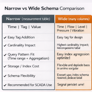
3.1 Data modeling: “narrow” vs “wide”
Two common schema approaches exist in SCADA:
- A) Narrow (measurement table): (time, tag_id, value, quality, status)
- B) Wide (many columns per row): (time, kW, flow, gate, vibration, …)
In practice, as the number of SCADA tags grows, a wide layout becomes difficult to manage. A narrow layout makes adding new tags easier and better matches time-series workloads. The trade-off is that it requires correct indexing and correct partition/chunk tuning. In the Timescale ecosystem, decisions such as “single hypertable vs multiple tables” matter for this reason [5].
3.2 Partition/Chunk strategy
Time-based partitioning is the foundation of query performance. In PostgreSQL, partitioning splits a table by a partition key, and “partition pruning” can exclude irrelevant partitions from a query [2]. In Timescale documentation, the chunk-interval concept is described as automatically splitting time series into chunks [1].
How do we choose chunk/partition size?
- Too small: Too many chunks → metadata/maintenance overhead.
- Too large: More scanning per query → higher latency.
Typical SCADA practice: 1–7 day chunks for raw data; larger intervals for summarized data.
3.3 Retention: “How long do we keep data?”
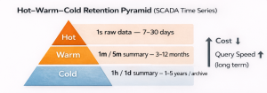
Keeping SCADA data as raw forever is expensive. TSDB approaches generally apply a hot–warm–cold pyramid:
- Hot: raw, second-level data (7–30 days)
- Warm: 1 min / 5 min summaries (3–12 months)
- Cold: 1 hour / 1 day summaries (1–5 years or archive)
InfluxDB documentation clearly explains downsampling + expiry via retention policies and continuous queries [3][4]. The same idea can be applied on the Timescale side with continuous aggregates plus retention/compression policies; policies can be defined on hypertables/continuous aggregates [6].
3.4 Downsampling: “Summarize raw data”
Downsampling converts older raw data into lower-resolution summaries. For example:
- 1-second raw → 1-minute avg/max/min
- 1-minute → 1-hour average + percentiles
This yields:
- Faster dashboard queries (fewer rows).
- Lower storage cost.
- Readable long-term trends.
3.5 Compression: “Compress old chunks”
Because time-series data is often append-only, “old data” rarely changes—ideal for compression. In the Timescale ecosystem, mechanisms like compression and compression policies can automatically compress older chunks [6].
Risk Box: Most common TSDB design mistakes
- Keeping raw data indefinitely (cost explosion).
- Not controlling cardinality (tag/label explosion).
- Choosing chunk interval randomly (too small or too large).
- Creating indexes for everything (hurts write performance).
- Collecting data without time synchronization (NTP/PTP) (timestamp drift).
(Basis: partitioning/retention principles [2][3][4])
4) SCADA query types: Four primary usage patterns that drive design
4.1 “Last X minutes” real-time trend
Operator screens and alarm dashboards typically query the last 5–30 minutes. For these queries:
- Index: (tag_id, time DESC) or time-focused index
- Chunk: small but not too small (1 day is a good starting point)
- Cache: short-lived cache at the dashboard layer
4.2 “Aggregation over a time range”
For KPIs (average power, daily flow, max vibration), a typical pattern is:
- WHERE time BETWEEN …
- GROUP BY time_bucket(…) / date_trunc(…)
Downsampling/continuous aggregates make a major difference here.
4.3 “Post-alarm forensic investigation”
You often want multi-tag correlation in a 10–30 minute window before/after an alarm. These queries involve:
- Many tags → high cardinality
- Narrow time window → indexing becomes critical
Grouping tags by unit and optimizing queries are important for this workload.
4.4 “Long-term reporting and comparisons”
Monthly/yearly reports must read from summary tables instead of raw data; otherwise billions of rows are scanned. This is why the retention + downsampling pyramid is essential [3][4].
5) Example scenario: Building TSDB design step-by-step for a hydropower plant
Assumptions:
- 1,500 tags
- On average 1 measurement per second per tag (1 Hz)
- Daily rows ≈ 1,500 × 86,400 = 129,600,000 rows/day
At this scale, a single-table approach quickly struggles. With a TSDB approach, you can apply the following plan:
Step 1 — Measurement schema (narrow)
measurements(time, tag_id, value, quality)
Index: (tag_id, time) and time-based partition/chunk [2].
Step 2 — Chunk interval selection
Use 1-day chunks for raw data (operational queries over last 30 days). Rationale: day-based maintenance and pruning convenience.
Step 3 — Retention plan
- Hot (raw, 1 second): 30 days
- Warm (1-minute summaries): 12 months
- Cold (1-hour summaries): 5 years
Step 4 — Downsampling rule
Before deleting data older than 30 days, produce 1-minute and 1-hour summaries.
Follow the “summarize first, then expire” logic as in InfluxDB RP + CQ [3][4].
Step 5 — Compression
Compress chunks older than 30 days; queries are rare but still possible when needed [6].
Figure 1 — Hot–Warm–Cold retention pyramid (raw short, summaries long).
Caption: Long-term storage cost is controlled while reporting performance is preserved.
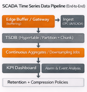
Figure 2 — SCADA measurement pipeline: Edge buffer → TSDB ingest → Continuous aggregates → Dashboard/Alarm screens.
Caption: Shows an end-to-end flow that reduces data loss under outage scenarios.
6) Hydrowise / Renewasoft approach: “SCADA data is not only stored—it is operated”
In Hydrowise, you can think of time-series handling in three layers:
1) Data layer (ingest + quality)
- Tag stream via OPC UA/SCADA integration
- Timestamp standardization (NTP/PTP)
- Quality flags (quality) to separate “trustworthy measurements”
2) TSDB layer (performance + cost)
- Time-based splitting via hypertable/chunk or PostgreSQL partitioning logic [1][2]
- Retention + downsampling plan (hot–warm–cold) [3][4]
- Compression and archival policies [6]
3) Product layer (operational value)
- KPI dashboard (kW, flow, efficiency, vibration trends)
- Alarm screens and event investigation
- Feature extraction for maintenance/failure analytics (feature-store mindset)
Internal link suggestions (site):
- /hydrowise/scada-entegrasyonu
- /hydrowise/gercek-zamanli-izleme
- /hydrowise/predictive-maintenance
- /renewasoft/ot-guvenligi
External authority sources:
- PostgreSQL Table Partitioning (official docs) [2]
- InfluxDB Downsampling & Retention Guide (official docs) [3]
7) Info card: “TSDB design checklist”
- Do you have time synchronization (NTP/PTP)?
- Is tag inventory and cardinality controlled?
- Was chunk/partition interval tested?
- Is the retention pyramid defined (hot–warm–cold)?
- Do you have downsampling jobs/continuous aggregates?
- Are indexes aligned to query patterns?
- Are backfill and outage scenarios planned?
- Monitoring: are write rate, disk usage, query latency, and bloat measured?
(Basis: partitioning and retention principles [2][3][4])
8) Frequently asked questions (FAQ)
1) Is Timescale/TSDB mandatory?
Not strictly, but without time-based partitioning and retention planning it is difficult to sustain performance for second-level SCADA streams [2][3].
2) What should the chunk interval be?
There is no single correct value. For raw data, 1–7 days is common. The best choice is determined by testing against write rate, query patterns, and maintenance cost [1][2].
3) How many days should I keep raw data?
It depends on operational needs. In practice, 7–30 days raw plus longer-term summaries is common [3][4].
4) What can downsampling break?
If aggregations are chosen incorrectly, short spikes can disappear. Keep max/min and percentiles as part of the summaries.
5) Do “bad actor” (noisy) tags affect TSDB?
Yes. Frequently changing or faulty sensors increase write volume and impact both storage and queries. Separate monitoring and quality controls are recommended.
6) What is the most critical risk when moving SCADA data to the cloud?Time synchronization, data integrity, and OT security (segmentation, authorization, logging) must be handled together [7].
7) Is PostgreSQL partitioning enough, or is a dedicated TSDB required?
PostgreSQL partitioning is a strong foundation [2]. TSDB solutions can reduce operational effort by automating chunk management, compression, and continuous aggregates [1][6].
9) Conclusion and next steps (CTA)
As SCADA time-series data grows, it turns into a workload that stresses classic table designs. The solution is to design time-based partitioning (partition/chunk), a retention plan, and the downsampling pyramid together. This trio keeps real-time dashboards fast and controls multi-year archive cost [2][3][4].
Actionable next steps:
1) Inventory your tags and estimate daily row volume.
2) Define hot–warm–cold retention targets.
3) Choose a chunk/partition interval for raw data and test it on a pilot table.
4) Enable 1-minute and 1-hour summary tables (downsampling).
5) With Hydrowise, align indexes and summary strategy with the query patterns of your KPI dashboards and alarm screens.
References
[1] TigerData (Timescale). Hypertables documentation. 2025. (https://www.tigerdata.com/docs/use-timescale/latest/hypertables) Accessed: 2026-02-22
[2] PostgreSQL Global Development Group. Table Partitioning (DDL Partitioning). 2025. (https://www.postgresql.org/docs/current/ddl-partitioning.html) Accessed: 2026-02-22
[3] InfluxData. Downsampling and Data Retention (InfluxDB documentation). 2016. (https://archive.docs.influxdata.com/influxdb/v1.0/guides/downsampling_and_retention/) Accessed: 2026-02-22
[4] InfluxData. Downsampling and Data Retention (InfluxDB documentation). 2015. (https://archive.docs.influxdata.com/influxdb/v0.11/guides/downsampling_and_retention/) Accessed: 2026-02-22
[5] TigerData (Timescale). Best Practices for Time-Series Data Modeling (hypertables vs multiple tables). 2024. (https://www.tigerdata.com/learn/best-practices-time-series-data-modeling-single-or-multiple-partitioned-tables-aka-hypertables) Accessed: 2026-02-22
[6] TigerData (Timescale). add_compression_policy() documentation. 2025. (https://www.tigerdata.com/docs/api/latest/compression/add_compression_policy) Accessed: 2026-02-22
[7] Stouffer, K. et al. NIST SP 800-82 Rev. 3 — Guide to Operational Technology (OT) Security. 2023. (https://csrc.nist.gov/pubs/sp/800/82/r3/final) Accessed: 2026-02-22