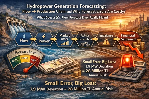
What Does a 5% Flow Forecast Error Really Mean?
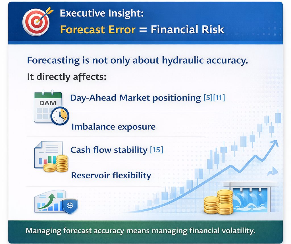
For a hydropower plant (HPP), generation forecasting may look like “just estimating MW from flow,” but in real operations it becomes a critical business input that directly determines the accuracy of Day-Ahead Market (DAM) offers, reservoir operating decisions, and imbalance costs.
A 5–10% deviation in flow forecasting does not only disrupt the production plan; it can also amplify settlement deviations, affect collateral requirements, and rapidly increase financial risk due to the hourly volatility of the System Marginal Price (SMP).
That is why a seemingly “small” hydraulic error can grow along the following chain and turn into real cost:
Flow → Power → Market Offer → Actual Generation → Imbalance → Financial Settlement
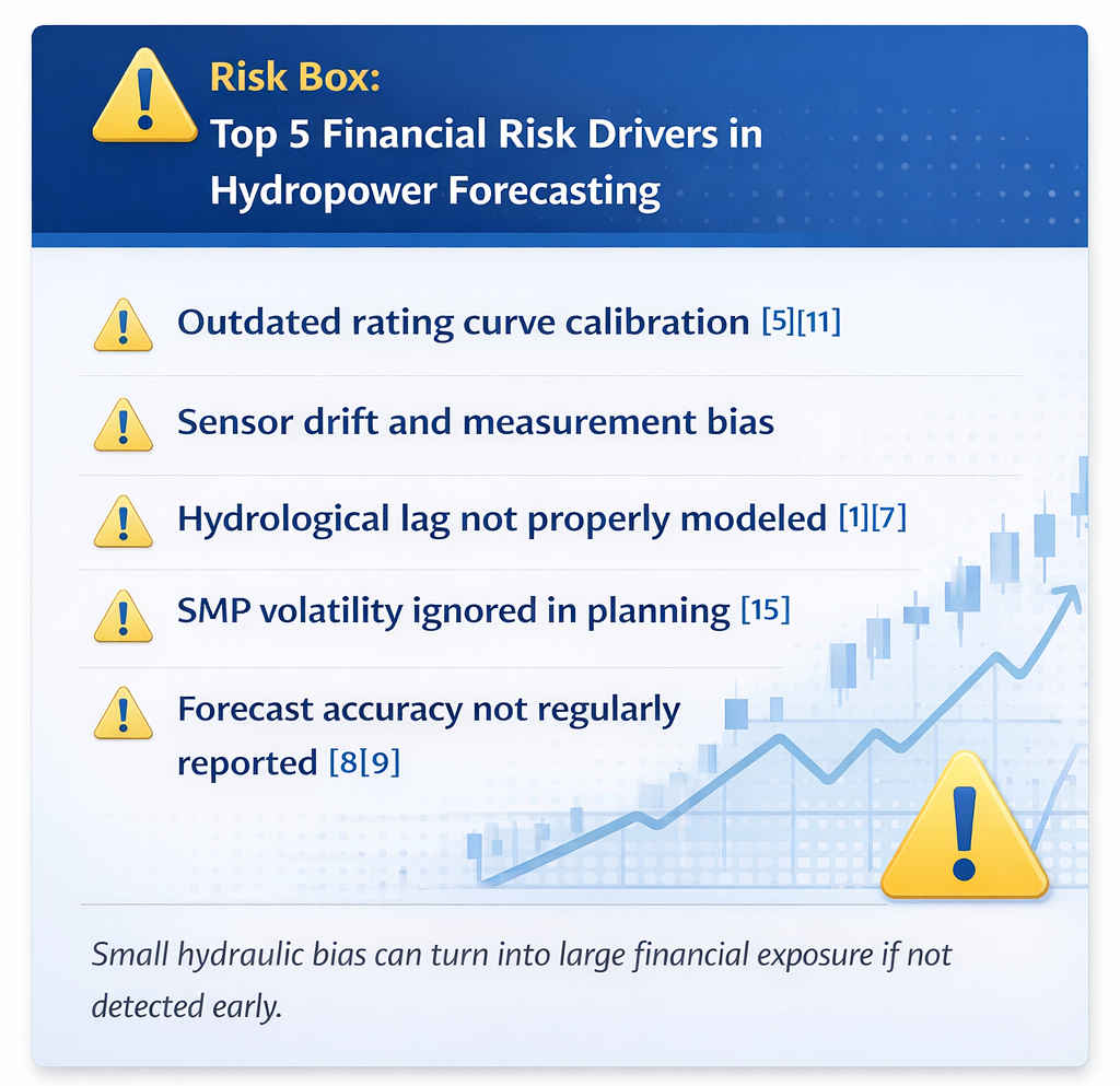
- Hydropower generation is fundamentally described by yet Q, H, and η are not constant in practice.
- Flow forecasting is affected by the stage–discharge rating curve (level-to-flow conversion) and measurement uncertainties.
- Rainfall–runoff response is delayed; hydrological modeling and calibration play a critical role.
- Forecast errors become monetary losses through SMP dynamics and the settlement/imbalance mechanism.
- Financial risk cannot be managed unless forecast accuracy is monitored regularly using metrics such as RMSE/MAPE/MASE.
Technical Foundations of Hydropower Generation Forecasting
Physical Basis of the Flow–Generation Relationship
At the core of hydropower generation is the following relationship:
- Q (Flow / Discharge): the water flow passing through the turbine
- H (Net head): effective head varying with reservoir level and hydraulic losses
- η (Efficiency): overall turbine + generator efficiency (varies by operating point)
This formula explains why and through which variables generation changes. However, because each parameter is dynamic in practice, forecasting becomes inherently challenging.
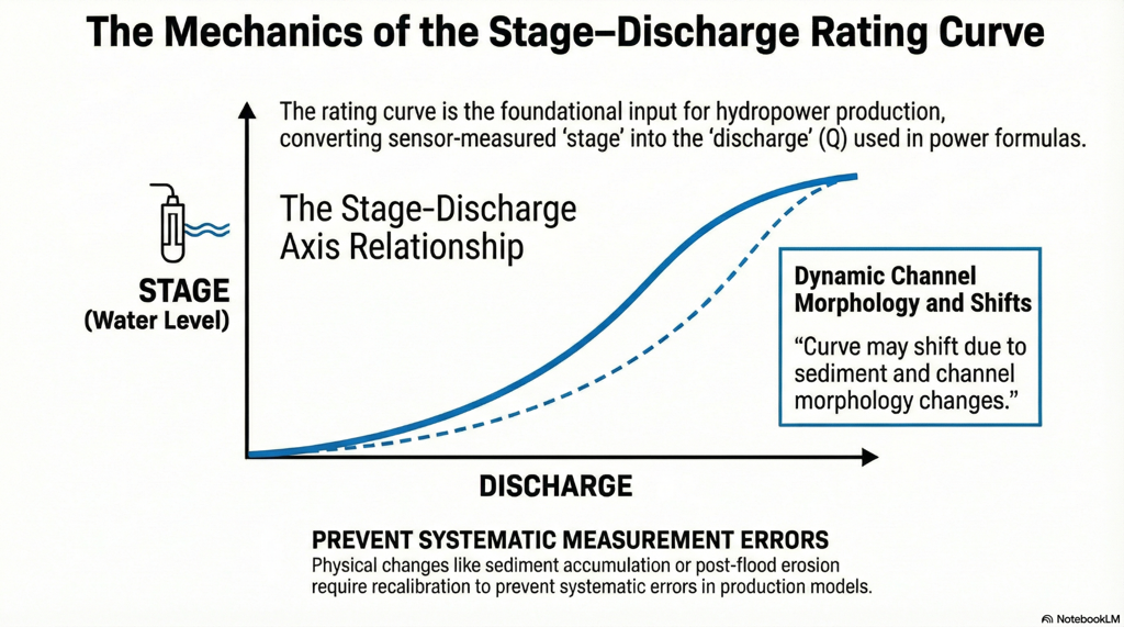
Rating Curve and Measurement Uncertainty
In most sites, flow is not measured continuously and directly; instead, water level is measured and converted to flow using a rating curve. Over time, this curve may drift due to cross-section changes, sediment accumulation, or post-flood morphological shifts—introducing systematic error into the model input.
Hydrological Lag and Modeling
When rainfall occurs, turbine inflow does not increase immediately. Catchment processes (infiltration, snow storage, evaporation, soil moisture dynamics) create a lag. Models such as HBV represent this transformation, and studies in Türkiye highlight the importance of model selection and calibration for real-time runoff forecasting.
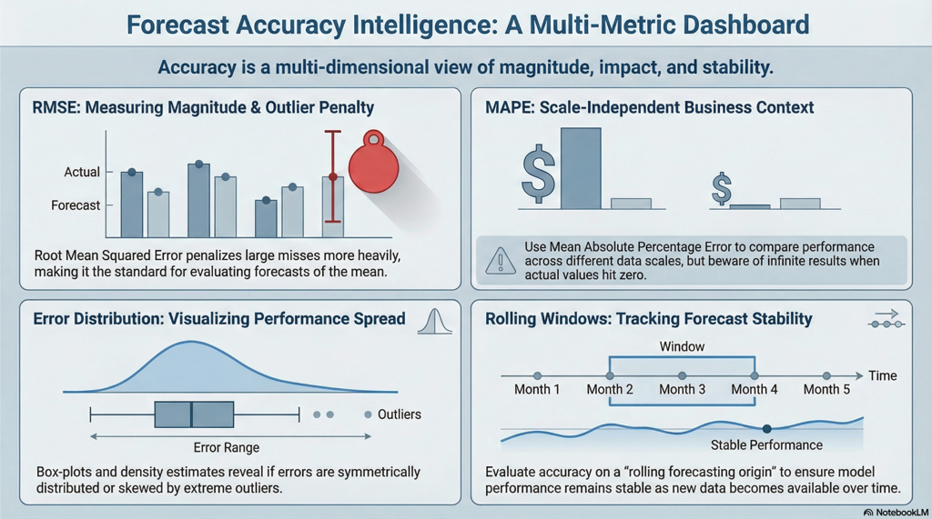
Measuring Forecast Performance
Tracking performance using only “average error” can be misleading. Hyndman’s work systematizes metrics such as RMSE/MAPE/MASE and principles for comparing forecasts. Operationally, the goal is not only to reduce error, but also to monitor error distribution and extreme deviations.
How Does Hydropower Generation Forecasting Work End-to-End? (H2)
In practice, hydropower generation forecasting operates end-to-end as follows:
- Data acquisition: SCADA/field sensors (level, gate position, turbine parameters) + meteorological inputs
- Flow derivation: level → flow conversion via rating curve
- Generation simulation: using accounting for the dynamics of H and η
- Forecast horizon: hourly/daily generation forecast aligned with DAM planning
- Bidding & planning: bidding strategy for the Day-Ahead Market
- Actual monitoring: actual generation and deviations
- Settlement: imbalance settlement under the balancing/settlement regulation; SMP impact
- Feedback loop: performance monitoring (RMSE/MAPE/MASE), drift control
Impact of Forecast Error on Plant Operations and Financial Performance
Within the plant, forecast error typically shows up as:
- Operational target deviation: daily generation targets are missed → intra-shift corrective pressure
- Reservoir strategy disruption: premature/incorrect water use → reduced flexibility for subsequent days
- Maintenance planning impact: forecasted production window is wrong → maintenance timing becomes harder
- Loss of financial visibility: risk is recognized “late” because the TL value of the deviation is not tracked clearly
- Penalty/additional cost risk: imbalance cost and collateral impacts may increase
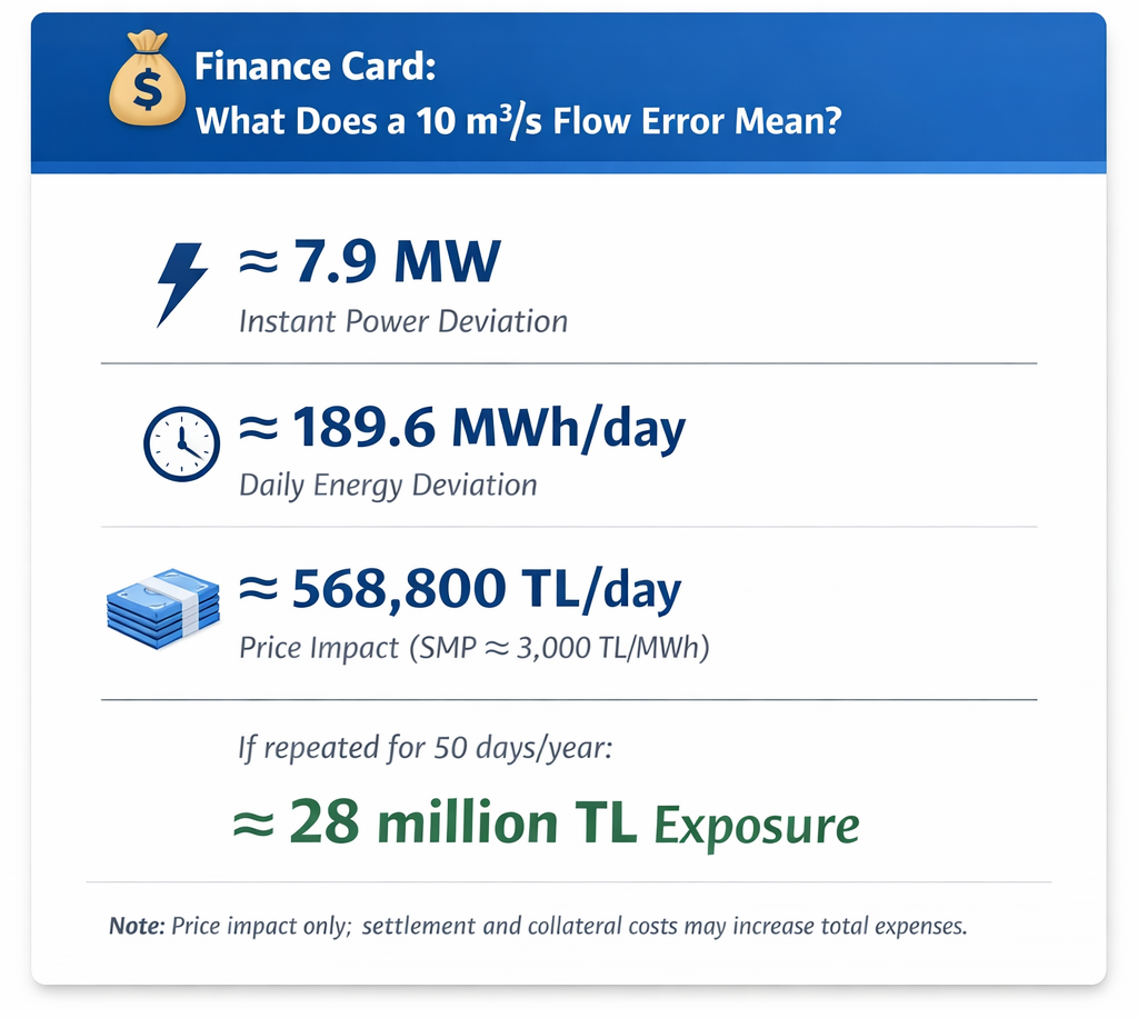
Numerical Example: Daily and Annual Financial Impact of a 10 m³/s Flow Error
The following example is a simplified calculation to illustrate how a “small” flow error can scale into a meaningful financial impact.
Assumptions
- Plant capacity: 50 MW (HPP scale)
- Average flow (Q): 80 m³/s
- Net head (H): 90 m
- Overall efficiency (η): 90%
- System Marginal Price (SMP): ~3,000 TL/MWh
Power Deviation (ΔP)
This corresponds to an approximate 7.9 MW instantaneous power deviation.
Daily Energy Deviation
This results in an approximate 189.6 MWh/day generation difference.
Daily Financial Impact
This is an approximate 568,800 TL/day price impact.
Annual Scale
If this repeats under similar conditions for 50 days in a year:
An approximate ~28 million TL financial risk can emerge.
Note: This calculation reflects price impact only; settlement rules, coefficients, and collateral processes may add further cost.
From Generation Forecasting to Financial Risk Management
In hydropower forecasting, the key challenge is not only predicting flow accurately. The critical question is whether the financial impact of forecast error is measured and integrated into decision-making.
In many plants, operations and market functions are managed separately. Operations teams focus on hydraulic accuracy, while trading teams handle the financial consequences of deviations. This separation often leads to delayed recognition of the true cost of forecast errors.
A data-driven approach addresses this gap by linking hydrological forecasting with market dynamics and financial outcomes.
This approach is typically built on three core principles:
Physical consistency
Flow forecasting should not rely solely on historical regression. Meteorological inputs, catchment response, reservoir levels, and turbine performance characteristics must be evaluated together to reflect real system behavior.
Continuous performance monitoring
Forecast accuracy must be tracked regularly. Metrics such as RMSE and MAPE should be treated as operational indicators, helping teams understand error behavior and detect extreme deviations early.
Market integration
Generation forecasts should be evaluated together with market conditions. Not only MW deviations but also their financial impact should be monitored. This allows early visibility of imbalance risk, collateral exposure, and planning decisions aligned with market signals.
Operationally, this approach supports:
• more consistent daily production planning
• reduced unexpected deviations
• improved financial visibility
• more controlled imbalance cost
Forecasting becomes part of a decision-support process rather than a standalone technical output.
Frequently Asked Questions (FAQ)
1) Why is flow forecasting critical for HPP operations?
Because flow forecasting directly impacts not only generation quantity but also DAM bids, reservoir strategy, and imbalance risk. Even small deviations can translate into financial outcomes.
2) Why is the rating curve so important?
In many plants, flow is derived from water level. If the rating curve is not updated, systematic error may occur, propagating into the model input and continuously biasing generation forecasts.
3) How do net head and turbine efficiency affect forecast accuracy?
Net head depends on reservoir conditions; turbine efficiency varies by loading. The flow–generation relationship is not perfectly linear, and ignoring this dynamic structure leads to unavoidable deviations.
4) Which metrics should we use to monitor forecast accuracy?
In operations, RMSE, MAPE, and error distribution should be evaluated together. Extreme deviations can disproportionately increase financial risk.
5) Why do forecast errors become “expensive”?
Because production deviations are settled under the balancing/settlement framework. Hourly SMP volatility can enlarge the TL value of deviations, and collateral processes may add further burden.
6) Where should we start for the fastest improvement?
Quick wins often come from: checking rating-curve validity, improving sensor calibration discipline, and regularly reporting forecast accuracy.
7) Do deep learning methods (e.g., LSTM) really make a difference?
Some studies report improved performance in hydropower forecasting. However, without data quality, monitoring, and continuous updating, changing the method alone is not sufficient.
8) What is the most critical question for an HPP operator?
Are you regularly measuring the TL value of forecast error? If forecast accuracy is not tracked together with financial risk, operational deviations are noticed late and the cost can grow.
Conclusion: Managing Forecast Error as Financial Risk
Hydropower generation forecasting is not only an engineering calculation. Flow forecasting is a critical decision input that directly affects plant financial performance—ranging from reservoir management and DAM bidding to imbalance cost and cash flow.
The chain discussed in this article highlights a clear reality:
- flow uncertainty cannot be fully eliminated,
- rating-curve and measurement errors can create systematic bias,
- hydrological lag increases complexity,
- SMP volatility can amplify small production deviations,
- even a seemingly limited deviation such as ±10 m³/s can create million-TL-scale risk.
The key takeaway is: Forecast error is not a technical problem—it is financial risk. So the right question is not “Do we have forecast error?” but:
“Do we measure and manage the financial value of this error on a regular basis?”
A 5% error may look small, but for a MW-scale plant, it can translate into a million-TL-scale impact over a year. Forecasting does not only mean “more accurate calculation”; it also means more controlled risk, more predictable cash flow, and a stronger market position.
If you would like to learn more about hydropower generation forecasting and managing forecast error as financial risk, feel free to contact us: