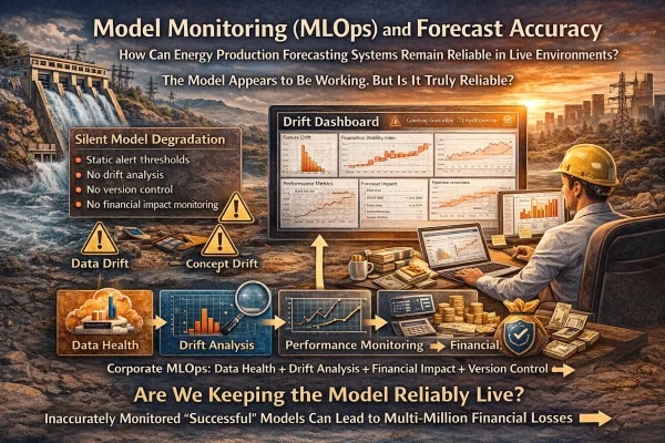
How Can Energy Production Forecasting Systems Remain Reliable in Live Environments?
The Model Appears to Be Working. But Is It Truly Reliable?
A production forecasting model deployed in a hydropower plant may initially demonstrate high accuracy. Achieving 90% accuracy on training data, low MAE, and stable performance charts can satisfy technical teams. However, three months later, the same model’s performance may gradually decline. The increase in error is not dramatic; therefore, no alert is triggered. The dashboard continues to operate. Reports are generated. Yet the model no longer accurately represents the physical system.
In the energy sector, forecast error is not merely a statistical deviation. The Day-Ahead Market operates on an hourly bid-matching mechanism [1]. Deviations in hourly production forecasts directly translate into balancing costs and revenue loss. Errors during peak hours generate disproportionately high financial impact. Therefore, model accuracy is not only a technical KPI but also a corporate risk indicator.
Machine learning models are mathematically static; however, the physical systems they represent are dynamic and evolving. For this reason, MLOps (Machine Learning Operations) forms the foundation of sustainable reliability in energy forecasting systems [2].
- Drift in energy forecasting systems is inevitable.
- Data drift and concept drift represent different risk categories [3].
- Average error metrics alone are insufficient.
- Silent model degradation may result in multi-million financial losses.
- Corporate MLOps requires data health monitoring, drift analysis, financial impact modeling, version control, and human approval.
Concepts and Background: Drift, Stationarity, and Energy Systems
Energy production forecasting systems are typically trained on historical data. This approach assumes statistical stationarity. However, real-world hydrometeorological processes are inherently non-stationary.
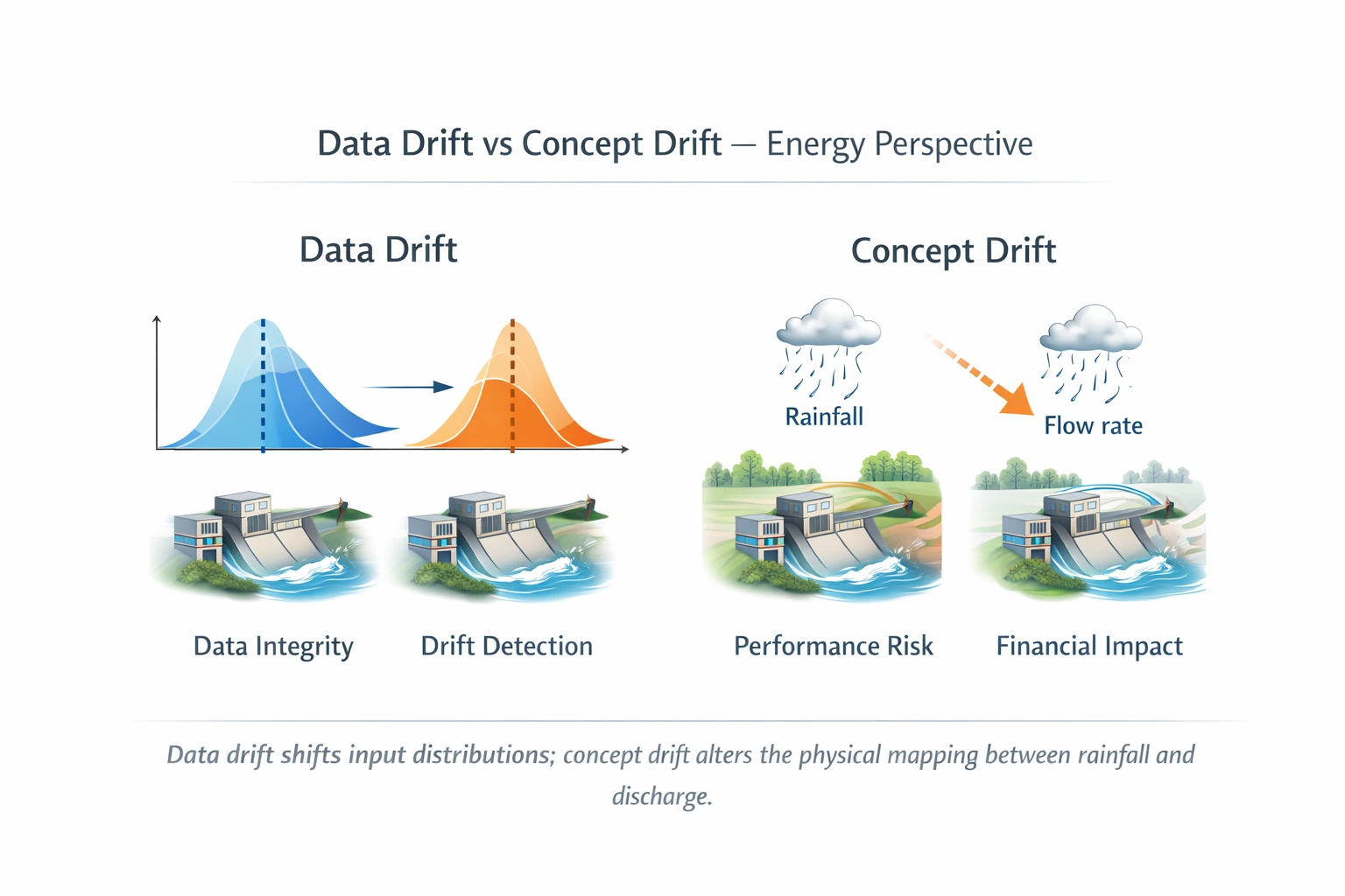
Model drift can be examined under two primary categories: data drift and concept drift.
1. Data Drift
Data drift refers to changes in the statistical distribution of input variables. For example, an increase in the frequency of extreme precipitation events [4] may cause deviation from the distribution observed during training. In such cases, the model continues to assume historical distribution characteristics.
2. Concept Drift
Concept drift is more profound. It occurs when the relationship between inputs and outputs changes over time [3]. The same rainfall amount may no longer produce the same discharge. Possible causes include:
- Changes in soil saturation structure
- Sediment accumulation
- Increased channel roughness
- Basin land-use transformation
Concept drift represents a loss of physical representativeness.
3. Mathematical Interpretation of Concept Drift
A machine learning model learns the relationship:
P(Y | X)
Under concept drift conditions, the conditional probability distribution changes over time:
Pt(Y | X) ≠ Pt+1(Y | X)
This situation may require not only retraining but also re-evaluation of the model architecture [3].
🔎 TECHNICAL NOTE
The Illusion of Statistical Stationarity in Energy Forecasting Systems
- According to the IPCC, the frequency of extreme weather events is increasing [4].
- Climate variability introduces long-term structural shifts.
- Energy infrastructure degrades over time, leading to performance loss.
Therefore, statistical stationarity assumptions are unreliable in long-term energy forecasting.
How It Works — Energy-Specific MLOps Architecture
A corporate MLOps architecture in the energy sector should consist of four primary layers: data health, distribution analysis, performance monitoring, and financial impact assessment.
1. Data Health Layer
This layer monitors:
- SCADA sensor anomalies
- Missing data ratios
- Timestamp synchronization issues
The NIST AI Risk Management Framework emphasizes data quality as a core element of AI risk management [5].
2. Distribution Analysis Layer
Feature drift is detected using methods such as:
- Population Stability Index (PSI)
- Kolmogorov–Smirnov test
- Adaptive Windowing algorithms [6]
A PSI value above 0.25 indicates significant distribution shift.
📌 Info Card
PSI Interpretation Range:
| 0.00–0.10 → Stable |
| 0.10–0.25 → Moderate change |
| 0.25 → Critical drift |
Source: [6]
3. Performance Metrics Layer
Traditional metrics such as MAE, RMSE, and MAPE are monitored [7]. However, in energy production forecasting, additional metrics must be evaluated:
- Peak Error (%)
- Lag Error (hour-based timing shift)
In hourly bidding systems, timing misalignment creates financial risk [1].
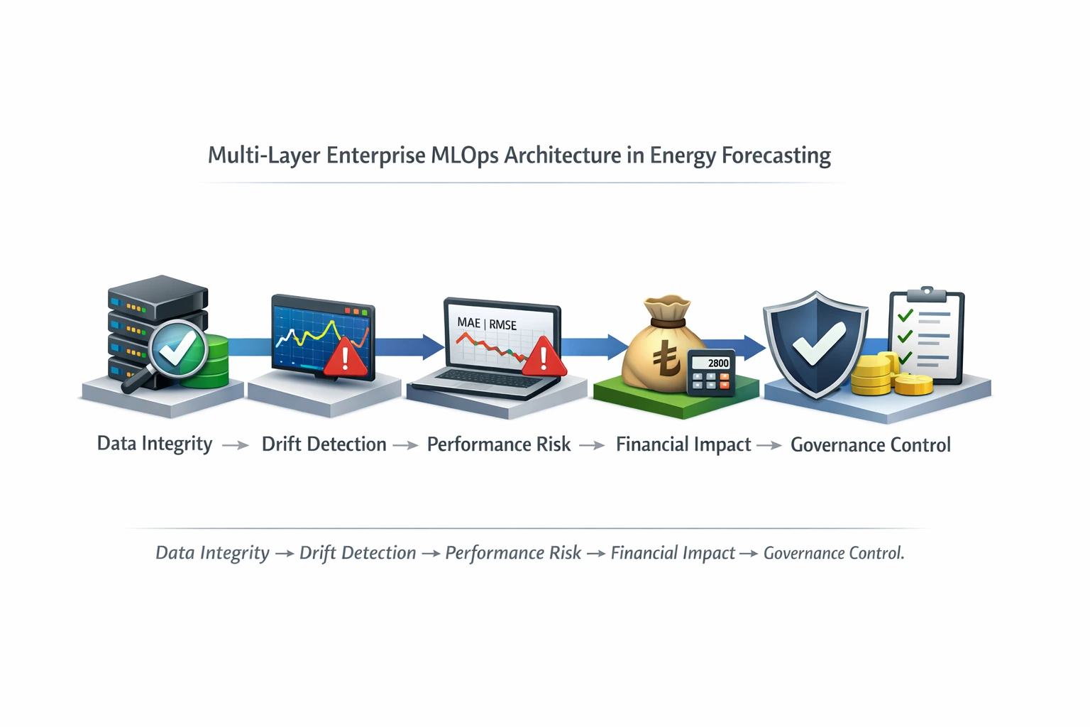 Figure 1
4. Financial Impact Layer
The financial impact layer simulates the revenue consequences of forecast error. This transforms model accuracy from a purely technical metric into a corporate risk indicator.
Example:
Forecast deviation: 8%
Peak price: 2800 TL/MWh
Deviation duration: 3 hours
The financial impact may be more significant than the statistical error magnitude. Without this layer, MLOps remains technical monitoring only.
Impact on Hydropower Plants
In a hydropower plant, discharge forecast error translates directly into production forecast error. Production forecast error directly affects Day-Ahead Market bidding strategy [1]. Due to hourly clearing mechanisms, errors during peak hours may grow disproportionately in financial terms.
For example, underestimating peak discharge by 20% may result in missed turbine optimization and potential revenue loss. Therefore, the forecasting system is not merely a technical component but also a financial reliability element.
The operational chain is as follows:
Discharge Forecast → Production Plan → Market Bid → Actual Generation → Balancing Cost
⚠️ Risk Card
Silent Model Degradation
- Static alert thresholds
- No drift analysis
- No version control
- No financial impact monitoring
Such a structure generates corporate risk.
Example Scenario / Mini Calculation
In a 65 MW hydropower plant over the last 120 days:
- MAE increased from 10% to 21%
- Peak error increased from 18% to 42%
- Lag error increased from 1 hour to 3 hours
Because the alert threshold was defined only as MAPE > 30%, no warning was triggered.
The operational outcome included underbidding during three major flow events and an estimated 2.2 million TL revenue loss. The model remained technically functional, yet the forecasting system was no longer revenue-secure. This illustrates the difference between operational status and financial safety.
Enterprise MLOps Approach in Energy Forecasting
The primary challenge in energy forecasting systems is not only achieving high model accuracy, but ensuring that this accuracy remains reliable over time.
In many organizations, model development and operational usage are separated. Data science teams focus on model performance, while operations teams face the financial consequences of forecast errors. This separation often delays the recognition of true model risk.
An enterprise MLOps approach bridges this gap by integrating model performance, data quality, drift behavior, and financial impact into a unified decision framework.
This approach is typically built on four core principles:
Data reliability
The quality of input data must be continuously monitored. Sensor anomalies, missing data, and timestamp inconsistencies directly affect model accuracy.
Drift monitoring
Data drift and concept drift must be regularly analyzed. Without tracking the deviation between training and live data distributions, model reliability cannot be sustained.
Performance evaluation
Traditional metrics such as MAE, RMSE, and MAPE must be monitored. However, in energy systems, peak error and timing misalignment (lag error) are equally critical.
Financial impact visibility
Forecast error should be evaluated not only statistically but also financially. This transforms model accuracy into a corporate risk indicator.
Through this structure, forecasting systems evolve from static models into monitored, measurable, and actively managed operational components.
Decision Layer: When Should a Model Be Considered Unreliable?
In MLOps systems, the most critical question is not whether a model is running, but when it should no longer be trusted.
In energy production forecasting, the following conditions should be treated as signals of model confidence loss:
• Peak error > 25% (especially during peak hours)
• Lag error > 2 hours
• PSI > 0.25 in critical features
• A consistent upward trend in error metrics (not sudden spikes)
In such cases, the system should:
1) Flag model outputs as low confidence
2) Shift operational planning to a conservative mode
3) Enable manual intervention when necessary
This approach transforms the model from a passive monitoring tool into an active decision-support component.
From Forecast Error to Decision Impact
In energy markets, forecast error is not only a financial loss but also a source of incorrect decision-making.
For example:
• Underestimation of generation → leads to underbidding
• Overestimation of generation → leads to imbalance costs
Therefore, MLOps systems should analyze not only the magnitude of error but also its direction.
Without bias (systematic error) analysis, model performance evaluation remains incomplete.
The Biggest Real-World Problem: Silent Drift
In energy systems, the greatest risk is not complete model failure, but gradual loss of reliability.
This typically occurs during:
• Seasonal transitions
• Extreme weather events
• Changes in basin behavior
For this reason, MLOps systems must go beyond threshold-based alerting and incorporate trend-based monitoring.
Otherwise, the model may appear to be functioning while continuously generating financial losses.
Frequently Asked Questions
- How often should a model be retrained?
In energy production forecasting systems, retraining should not be performed at fixed time intervals. Instead, it should be triggered by changes in model performance and data behavior.The following conditions typically indicate the need for retraining:
• PSI > 0.25 in critical features
• Peak error > 25% (especially during peak hours)
• A consistent upward trend in error metrics (7–14 days)
• Emergence of a new hydrometeorological regime (e.g., extreme rainfall season)Therefore, the most effective approach is not time-based retraining, but a hybrid strategy driven by drift detection and performance degradation.
- Is MAPE sufficient?
No. MAPE reflects average error magnitude, but in energy systems, extreme events and peak conditions are far more critical.The following metrics should be evaluated together:
• Peak Error (%) → error during high-impact hours
• Lag Error (hour-based) → timing misalignment
• Bias → systematic over- or under-estimationIn hourly bidding systems, timing misalignment (lag error) may create greater financial risk than average error levels.
- Does drift always imply model failure?
No. When drift is detected, the first step should be to validate data quality rather than assuming model failure.Drift may be caused by:
• Sensor anomalies
• Missing or delayed data
• Timestamp synchronization issues
• Structural system changes (concept drift)Therefore, drift analysis must begin with data validation before evaluating model behavior.
- Is fully automated retraining safe?
In critical infrastructure systems (especially energy and SCADA environments), fully automated retraining is generally not recommended.This is due to:
• The risk of training on corrupted or low-quality data
• Unexpected changes in model behavior
• Uncontrolled impact on operational processesThe safest approach is:
Human-in-the-loop retraining, where model updates require expert validation.
- Why is AI governance important?
Energy forecasting systems are not just technical tools; they are operational and financial decision systems.Therefore, it is essential to ensure:
• Full traceability of model versions
• Proper documentation of training datasets
• Approval mechanisms for model changesRegulatory frameworks such as the EU AI Act and ISO AI standards require monitoring, traceability, and governance mechanisms in critical systems [9][10].
This approach elevates model accuracy from a technical metric to a corporate reliability standard.
Conclusion
An energy production forecasting system is not merely an analytical tool but an operational asset. Model accuracy is directly linked to financial stability and operational security. Drift is inevitable; an unmonitored model will gradually lose reliability.
If you would like to learn more about MLOps and maintaining reliable forecasting systems in energy operations, feel free to contact us: